Close Enough

Back in October, Greg Wilson blogged about testing scientific software. He specifically points to a lesson introducing the Euler method as part of the Practical Numerical Methods with Python MOOC, and asks why a certain number (the measured convergence rate) is close enough to the expected value.

The big question of testing in scientific software, how this should be done, and how it is being done, has led to the Close Enough for Scientific Work project, as launched and explained by Greg Wilson in this blog post. If you're reading this, you should be following that project! As I've helped out on the MOOC, which is led by Lorena Barba, I've been (over)thinking what sort of answer we could, or should, give. Well aware that we're heading for the academic version of the balloon joke (an answer that is correct, of little use, and took a long time to arrive), I've outlined some answers in the posts linked below.

Background¶

$$ \newcommand{\dt}{\Delta t} \newcommand{\udt}[1]{u^{({#1})}(T)} $$

We have a system of differential equations to solve: the solution will be $u(t)$. The numerical solution we get will depend on one parameter, the timestep $\dt$. The resulting numerical approximation, at the point $t=T$, will be $\udt{\dt}$: the exact solution is $u(T)$.

The method used is Euler's method, also introduced in an earlier lesson in the MOOC, and explained in detail by Lorena in this screencast. The key result derived there is that Euler's method is first order, so that

$$ \begin{equation} u(T) - \udt{\dt} = c_1 \dt + c_2 \dt^2 + {\cal O}(\dt^3) \simeq c_1 \dt. \end{equation} $$

For sufficiently small $\dt$ the error is proportional to $\dt$.

As we can't (usually) know the exact solution $u(T)$ ahead of time, a standard check is grid convergence: compute three solutions with different timesteps (eg, $\dt, 2\dt, 4\dt$) and compare them. The comparison to use is

$$ \begin{equation} s_m = \log_2 \left( \frac{\udt{4\dt} - \udt{2\dt}}{\udt{2\dt} - \udt{\dt}} \right) \simeq 1. \end{equation} $$

The symbol $s_m$ is used as it's the (measured) slope of the best fit line through the errors, as shown on the original lesson:

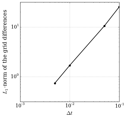
Figure 1. Convergence test plot taken from the original lesson.

The original lesson does precisely this comparison (using the phugoid model, with specific parameter values, and $\dt = 0.001$), finding a measured slope $s_m = 1.014$. Is this close enough to 1?

TL;DR: Answer¶

Answers

1. I don't care about the algorithm: I just want the answer to be right: $0.585 \lesssim s_m \lesssim 1.585$ is close enough for Euler's method.
2. I don't care about the answer: I just want the algorithm behaviour to be right: $s_m=1.014$ with $\dt=0.001$ is close enough if $1 \le s_m \le 1.0093$ with $\dt=0.0005$.
3. I don't care about the behaviour: I just want to know I've implemented Euler's method: measure the local truncation error instead, and check both the convergence rate and the leading order constant. $s_m$ by itself is useless.

And yet more¶

The accuracy of the convergence rate was just one small point in Greg's original post. The more substantial question was on testing a "real" code, such as this n-body simulation code. To illustrate how far you can go with the approaches described above, here's my attempt at testing that code.

Acknowledgements¶

Aside from the obvious debts to Lorena Barba and Greg Wilson, both for starting this off and for later comments, I've also benefitted from comments from and discussions with Hans Fangohr and Ashwin Srinath.