Bulk viscosity

Nuclear reactions, Bulk viscosity, Neutron Star mergers, and Gravitational Waves

Ian Hawke
P Hammond, T Celora, M Hatton
J Foster
N Andersson, G Comer

See 2205.11377, 2108.08649, 2107.01083
github.com/IanHawke
STAG, University of Southampton

ianhawke.github.io/slides/et-2023

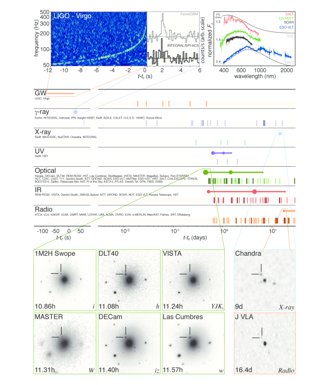
GW170817

One multimessenger detection.
- Gravitational waves;
- $\gamma$ - first detected;
- All EM band - long term.
GWs seen for inspiral.
Constrains matter properties.
- Masses;
- Tidal compressibility;
- Equation of state.
O4 just starting:
Many more detections.

How does parameter estimation work?

Parameter Estimation

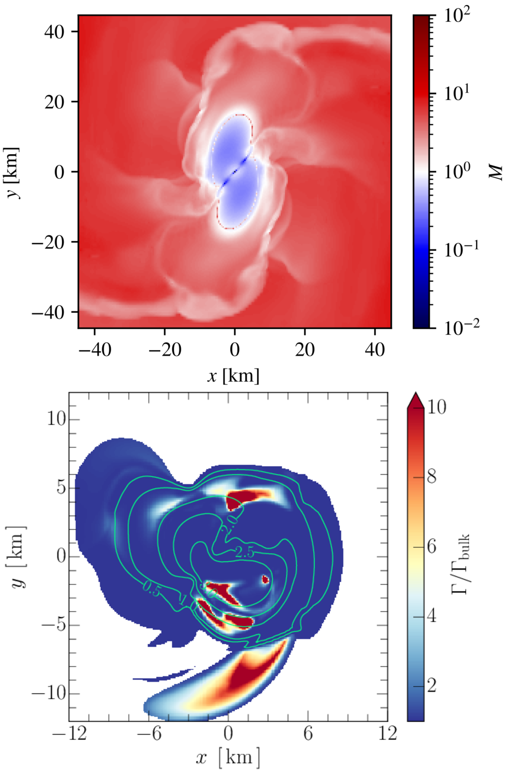
Neutron star merger

Merger is messy:
- Shearing instabilities;
- Temperature increase through shocks;
- Nuclear reactions.
Urca reactions: $$ \begin{aligned} \text{n} &\to \text{p} + \text{e}^- + \bar{\nu}_e \\ \text{p} + \text{e}^- &\to \text{n} + \nu_e. \end{aligned} $$
Keep track of species $Y_\text{e} \sim n_\text{e} / n_b$ by $$ D_t Y_\text{e} = \Gamma_\text{e}(n_b, T, Y_\text{e}). $$
Urca timescale $\sim 10^{-8}-10^{-10}$ seconds: $< \Delta t$. Stiff: $\Gamma_\text{e} \gg 1$.

There is a lot of physics driven by merger. Here the focus is on the small-scale structure driven by merger, with the shocks making the temperature shoot up, shearing instabilities and turbulent effects driving power to small scales, and neutrinos and nuclear reactions becoming much more important. Here I'm going to be motivated by the weak interactions, particularly of Urca type, where the relative amount of baryons and electrons changes due to the reactions, with energy-momentum transferred into neutrinos.
For now, the focus is on the evolution of the lepton fraction keeping track of the number of electrons at each point. This is an advection equation with a source - the reaction rate. The dimensions of the reaction rate are inverse time, so we need an idea of the reaction timescale.
Unfortunately for numerical studies, typical Urca reaction rates can be smaller than the numerical timestep. When we solve the evolution equations, we would want to use explicit methods: we can't do this stably. We're left with a problem: we can either switch to a timestep limited by the reactions or an implicit scheme in time, both of which are impractical. Or we can do something else.

Toy model

Approximate fluid equations, using $\theta = \nabla_a u^a$:

$$ D_t \begin{pmatrix} n_b \\ e \\ Y_\text{e} \end{pmatrix} = - \begin{pmatrix} n_b \theta \\ \left( e + p(n_b, e, Y_\text{e}) \right) \theta \\ {\color{red}\epsilon^{-1}} \left( A Y_\text{e} - B \right) \end{pmatrix}. $$

Short timescale encoded in $\epsilon \ll 1$.

Assume $Y_\text{e} = Y_0 + \epsilon Y_1 + \dots$ and separate scales:

$$ \begin{aligned} \mathcal{O}(\epsilon^{-1}) & \colon & 0 &= -A Y_0 + B & \implies & Y_0 = Y_\text{eq} = F(n_b, e), \\ \mathcal{O}(\epsilon^{0}) & \colon & D_t Y_0 &= -A Y_1 \\ & \implies & Y_1 &= -A^{-1} D_t Y_0 \\ & & &= G(n_b, e) \theta. \end{aligned} $$

Expand pressure:

$$ \begin{aligned} p(n_b, e, Y_\text{e}) &= p(n_b, e, Y_\text{eq}(n_b, e)) + \epsilon \partial_{Y_\text{e}} p Y_1 \\ &= p_\text{eq}(n_b, e) + \Pi, \\ \Pi &= -\zeta(n_b, e) \theta. \end{aligned} $$

Appearance of bulk viscous pressure.

Reduced model:

$$ D_t \begin{pmatrix} n_b \\ e \end{pmatrix} = - \begin{pmatrix} n_b \theta \\ (e + {\color{blue} p_\text{eq} + \Pi}) \theta \end{pmatrix}. $$

No longer tracking species: always in equilibrium.
Scales now tractable: $\Gamma_\text{e} \sim \epsilon^{-1} \to \Pi \sim \epsilon.$

We develop the key idea using a toy model.
Here we've taken the relativistic fluid equations and made a couple of key approximations. First, we've assumed we're working in coordinates moving along with the fluid flow. Second, we've assumed we're working on a small enough scale that the pressure and the expansion (which is the divergence of the velocity) are both roughly constant. There's plenty of cases where this doesn't work - turbulence wouldn't allow us to do this - but enough cases where it will to fix our ideas.
Next, we assume that the reactions are happening on a short timescale. Dimensionally we can pull this out into $\epsilon$, a small number encoding the ratio of scales. We will also linearize the reaction rate to make the steps clearer, although this isn't essential. Our key assumption is now that there is scale separation: behaviour at each power of $\epsilon$ is independent. Again, this wouldn't work in turbulent cases.
With these assumptions we can look for a power series solution in the species fraction. Plug this power series into the equation of motion for the species fraction and look at each power of the scale ratio separately. The leading order term in the power series is then fixed: remember $A, B$ are known functions that don't depend on the species fraction, as they come from linearising the reaction rate. We also see that this leading order term is in equilibrium: if it were the total species fraction and we plugged it into the equation of motion then its time derivative vanishes.
At zeroth order we have the next term in the expansion given by the time derivative of the equilibrium leading order term. Using the chain rule and the other equations of motion we can expand the time derivative. The precise form of the terms isn't essential here. What matters is that they are all evaluated at equilibrium, where the species fraction is given by the leading order term, which itself depends only on the baryon number and internal energy. We also pull out a factor of the expansion.
The reason for pulling out the expansion can be seen by going back to the other equations of motion, those for the baryon number and internal energy. The only place where the species fraction matters is in the pressure. We Taylor expand about equilibrium: the first order term is proportional to the first order term in the species fraction, so proportional to the expansion. That means it behaves exactly as expected for a bulk viscous pressure. The bulk viscous coefficient then depends on the baryon number and internal energy.
Putting this all together, what this multiscale calculation does is give us a reduced model. In the reduced model the species fraction is not evolved, but always assumed to be in equilibrium. Its value can be computed by setting the reaction rate to zero. The leading order impact of the out-of-equilibrium behaviour that should be there manifests itself as a bulk viscous pressure. The bulk viscous pressure coefficient can be evaluated using appropriate derivatives of the reaction rate, evaluated at equilibrium. We thus have to evaluate fewer equations of motion. More importantly, the problematic fast timescale has been removed from the problem, as the bulk viscous pressure correction term is linear in the small scale ratio, not inversely proportional to it as the reaction rate was.

Impact of $\Pi$

Check with a "real" equation of state:

Bulk viscous pressure can be big for neutron star core in merger;
Bulk viscous approximation needed above dashed lines (resolution dependent).

Let us now move from the toy model to looking at the impact for a real equation of state. Here we're using the APR4 equation of state, with the reaction rates and derivatives computed using the Fermi surface approximation. That's not ideal: unfortunately very few equations of state also have the reaction rates in a suitable form for this calculation in full.
This plot covers the range of densities and temperatures relevant for a neutron star merger. The core of the neutron star is typically at a few times nuclear saturation density (see note below). The outer layers of the neutron star are many orders of magnitude lower, but the Urca reactions are rapidly suppressed at low densities. The temperature of the neutron star during inspiral is low - it is expected to be well below 1MeV - but can reach around 100MeV through merger in extreme cases.
There are two key pieces of information in this plot. The first, given by the colour, is how big the bulk viscous pressure is compared to the total pressure. We see this can be substantial - certainly into the percent level - at low temperatures, and particularly through the core. The second piece of information is the timescale of the reactions. Remember, bulk viscous pressure is an approximation, and that approximation is only needed if the numerical timestep is too big. The lines pick a particular timestep. Every region below a line has reactions slow enough that the bulk viscous approximation isn't needed, and the full nonlinear reaction can be directly solved. The solid line is quite a poor numerical resolution by current standards. The top, dotted, line is an order of magnitude better than the best simulation ever run. We see that there's a region in parameter space where we will have no choice but to use a bulk viscous approximation.

Impact on GWs

Do nonlinear merger simulation;
Simulate with $\epsilon \to 0, \infty$;
Filter out inspiral signal;
Reactions "soften" EOS, $$\Delta f \simeq 58\textrm{Hz}$$
Compute the mismatch between signals, $$ \mathcal{M} \sim 1 - \frac{\max \langle h_1 \vert h_2 (\sim \textrm{phase}) \rangle}{\sqrt{\langle h_1 \vert h_1 \rangle\langle h_2 \vert h_2 \rangle}} $$
$$ \varrho_\textrm{req} \gtrsim 1 / \sqrt{2 \mathcal{M}} \quad = 1.2 $$ Limits are distinguishable in GWs by ET.

Having argued that the nuclear reactions, in the bulk viscous approximation, can be relevant through merger, we actually want to test that. Doing the full nonlinear simulations is a real pain: for proper consistency we would need to keep track of the products of the reactions - that would be the neutrinos - by including radiation hydrodynamics, which increases the computational expense massively. Instead we focus on the extreme limits: the case where the reactions are infinitely slow and infinitely fast. If there's no way of distinguishing between these two cases observationally then we can leave this out of the model.
The simulations here again use the APR4 equation of state, and take two 1.4 solar mass neutron stars, initially 40km separated and in equilibrium, and run the simulation through a few orbits before merger. The three gravitational wave signals you see here are the slow and fast reaction limits, and then the slow reaction limit again but with a different numerical resolution to check that any differences are due to changing the model, not numerical error. By eye, it's impossible to tell the difference between the models.
However, we don't quantify signals by eye, nor do we do it in the time domain. Instead we look at signals in the frequency domain. So, perform the Fourier transform and look at where the power is in the signal. As the inspiral phase of the simulation will be the same - reactions only do anything at high enough densities and temperatures, so in the post-merger regime - we filter out the lower frequency inspiral signal to concentrate on the post-merger behaviour. This filtering was done in two different ways, and the result are unchanged by the choice.
The top panel compares the power spectra of the two models. The horizontal line is the design noise curve for the Einstein Telescope, giving us confidence that this post-merger signal would be detectable in ET. The peak in the power spectra of the post-merger signal has moved, as shown by the vertical dashed lines, by about 60Hz. This isn't a lot in a signal at 3kHz, but is orders of magnitude more than the phase change caused by changing numerical resolution, shown in the bottom panel.
The question is then whether this makes a difference for estimating physical parameters in an observational pipeline. In particular, if we had a signal, and had the two templates for the different reaction limits, would we be able to distinguish which template was the better fit to the signal, given the noise? We can use the mismatch between the template signals to find the required signal-to-noise-ratio for distinguishability. The mismatch roughly finds the minimum difference, in frequency space, of two signals after phase and time shifting. The SNR required is then roughly the inverse square root of the mismatch. In our case the mismatch was 36%, so the SNR required is 1.2.
For a merger happening at a similar distance to GW170817, and using a next generation GW detector, we see that the signals are distinguishable.
I need to emphasise that this does not mean we could measure nuclear reaction parameters through GWs. We should instead think of this as being a potential systematic error in the signals. It's then necessary to include nuclear reactions correctly into numerical simulations to get sufficiently accurate templates for ET.

Solve the toy problem

Full problem:
Bulk viscous approximation:
"Infinitely fast" $\implies \Pi \to 0$.
${\footnotesize \zeta = \epsilon p_{,Y_\text{e}} A^{-1} \left( n_b Y_{\text{eq},n_b} + (e + p_\text{eq}) Y_{\text{eq}, e} \right) }.$

Check accuracy

Vary the fast timescale.
See the expected behaviour:
- Leading order error $\propto \epsilon$;
- Bulk viscous error $\propto \epsilon^2$;
- More terms including, better overall error.

Argues for the use of the bulk viscous pressure correction.

Start out-of-equilibrium

Previously $$ Y_\text{e}(t=0) = Y_\text{eq}(t=0), $$ equilibrium.
Now set $$ \begin{aligned} \Delta Y &= Y_\text{e}(t=0) - Y_\text{eq}(t=0) \\&= \mathcal{O}(1). \end{aligned} $$
$Y_\text{e} \to Y_\text{eq}$ exponentially, timescale $\epsilon^{-1}$.
$\Pi$ correction doesn't seem as accurate.

Check accuracy

Vary the fast timescale.
Do not see the expected behaviour:
- Leading order error $\propto \epsilon$;
- Bulk viscous error $\propto \epsilon$!
- Errors comparable.

What has gone wrong?

Did power series expansion $$ Y_\text{e} = Y_0 + \epsilon Y_1 + \dots $$
Cannot capture boundary layer - exponential term.

Boundary layers

Solution: rescale $\tau = t / \epsilon$.
Re-solve using $$ Y_\text{e} = \tilde{Y}_0(\tau) + \epsilon \tilde{Y}_1(\tau) + \dots $$
Captures exponential behaviour in $t$.
Matched asymptotics: $$ \tilde{e}(\tau=1) = e(t = \epsilon). $$
$\epsilon \ll 1$, match "changes initial data".
Simple fix: $$ e(t=0) \to e(0) - \epsilon A^{-1} \Delta Y p_{,Y_\text{e}} \theta. $$

Check accuracy

Vary the fast timescale.
Again see the expected behaviour:
- Leading order error $\propto \epsilon$;
- Bulk viscous error $\propto \epsilon^2$

Matched asymptotics and modifying the initial data mean we can successfully use bulk viscous approximations.

Within a numerical scheme, discrete steps or multi-physics aspects can act to push things out of equilibrium...

Summary

Neutron star mergers need nonlinear numerical simulations.
Timescales mean subgrid schemes/models required.
Interpret models as bulk viscous corrections.
Modelling reactions necessary to avoid systematic errors.

Look out for problems!

Coupling to full radiation hydro might give double counting issues.
Potential for boundary layer issues in numerical codes.

Hammond+; Most+.