2 Spectral methods
In previous chapters we have discussed the stability and accuracy of finite difference methods by looking at the impact in frequency space. This can be seen either as a Fourier transform, or as a function basis expansion as, for example, a complex Fourier series.
We could move from numerically solving the differential equation using finite differences to instead numerically solving the function basis expansion. This chapter outlines the key issues behind that approach, which is broadly called a spectral method.
2.1 Advection expansions
As usual we will start with the one dimensional linear advection equation (Equation 1.5) in the form
\[ \frac{\partial \phi}{\partial t} + u \frac{\partial \phi}{\partial x} = 0. \tag{2.1}\]
We assume the boundaries are periodic. We then approximate the solution as a truncated complex Fourier series
\[ \phi(x, t) = \sum_{k = -N}^{N} a_k(t) \exp(i k x) \, . \tag{2.2}\]
The time dependence is completely contains within the coefficients \(a_n(t)\), which determine the solution. The number of modes used in the approximation, \(2 N + 1\), controls the accuracy of the method, and can be thought to be like the number of grid points in a finite difference method.
The series expansion substituted into the advection equation (Equation 2.1) gives
\[ \sum_{k = -N}^{N} \left\{ \frac{\text{d} a_k}{\text{d} t} + i k u a_k \right\} \exp(i k x) = 0. \tag{2.3}\]
In the simplest case where \(u\) is a constant, the orthogonality of the complex exponentials decouples all the modes to leave the ordinary differential equations
\[ \frac{\text{d} a_k}{\text{d} t} + i k u a_k = 0. \tag{2.4}\]
This can be solved explicitly and exactly giving \(a_k = a_k(0) \exp(-i k u t)\). We therefore have the approximate solution
\[ \phi(x, t) = \sum_{k = -N}^{N} a_k(0) \exp[i k (x - u t)] \, . \tag{2.5}\]
This solution has no dispersion error (all information propagates exactly at speed \(u\)) and its amplitude is constant. The error comes from projecting the exact initial data onto the basis functions, using a truncated series. This can have odd effects when \(N\) is small - strictly positive functions can appear to go negative - but for smooth data these problems converge very rapidly (as Fourier series approximations converge rapidly).
2.2 Non-uniform advection
With finite difference and finite volume methods moving to non-uniform and nonlinear problems is “straightforward”, although their numerical analysis can be difficult. For example, if the advection velocity \(u\) is not constant so that \(u = u(x)\), the standard FTBS method (as seen earlier) is directly written as
\[ \phi^{n+1}_j = \phi^n_j - \frac{u_j \, \Delta t}{\Delta x} \left( \phi^n_j - \phi^n_{j-1} \right) \, . \tag{2.6}\]
The only change to the standard FTBS scheme is that the advection velocity is now evaluated at the update point, \(u_j = u(x_j)\). The CFL limit constraining the timestep now needs to maximize over all points \(x_j\), or equivalently over all advection velocities \(u_j\).
The spectral method, however, now becomes markedly more complex. As \(u\) varies in space we need to represent it by Fourier series expansion as well, as (for example)
\[ u(x) = \sum_{l = -N}^{N} u_l \exp(i l x) \, . \tag{2.7}\]
When we substitute the series expansions for both the solution and the advection velocity into the advection equation we get
\[ \sum_{k = -N}^{N} \left\{ \frac{\text{d} a_k}{\text{d} t} + i k a_k \sum_{l = -N}^{N} u_l \exp(i l x) \right\} \exp(i k x) = 0. \tag{2.8}\]
When we use orthogonality we find
\[ \frac{\text{d} a_k}{\text{d} t} + i \sum_{\substack{k+l = N \\ |k|, |l| \le N}} k a_k u_l = 0 \, . \tag{2.9}\]
This couples different modes (different values of \(k\)). We can no longer solve this ordinary differential equation exactly; instead we have to use some time differencing method to compute the result.
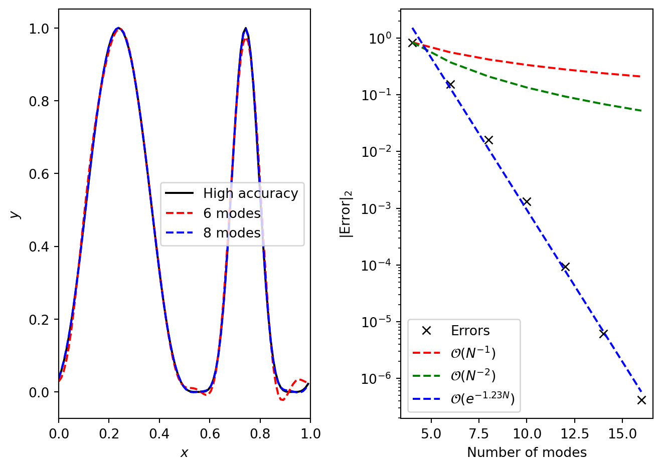
The results of applying a spectral method to non-constant advection can be seen in Figure 2.1. The left panel shows the solution after “half a period”, which is extremely well captured even with very few modes used (look at the solution near the right edge for the largest discrepancies). The convergence plot in the right panel is the key result, however. It shows how the error converges exponentially, which is far faster than any finite differencing scheme (which converges polynomially) can manage.
2.3 Problems and solutions
The fundamental lesson of spectral methods for complex, nonlinear systems is given by Equation 2.9. That is, the approximate solution is updated by coupling every mode of the solution at the current time. This leads to extremely high accuracy but is associated with high costs. In particular, there are \(\mathcal{O}(N)\) ordinary differential equations of the form (Equation 2.9) that need to be solved, and each requires \(\mathcal{O}(N)\) terms to be evaluated within the sum, so each timestep costs \(\mathcal{O}(N^2)\). For large numbers of coefficients this is much more expensive that a finite difference scheme.
Some of these costs can be ameliorated by performing the nonlinear (or non-uniform) calculations in position space rather than frequency space. That is, the terms in the product \(u \partial_x \phi\) can be Fourier transformed back to position space, multiplied, and then transformed back. This is cheaper, reducing the cost to \(\mathcal{O}(N \log N)\). This idea is linked to spectral collocation methods.
A related problem caused by all modes coupling is that of accuracy. When a mode with wavenumber \(N\) couples to another mode with wavenumber \(N\) then the true result should be a non-trivial evolution of the mode with wavenumber \(2N\). However, our truncated series approximation does not allow for this information to be captured. The information lost due to the nonlinear interactions at high wavenumber can have significant impacts, and particular techniques are needed to adjust for it. One standard method is to only use \(2/3\) of the coefficients when calculating the update terms. This (additionally) truncated approximation avoids aliasing problems due to the interactions.
Another, sometimes critical, problem, is related to the use of a single function basis expansion over the entire domain. In the example above we used a Fourier series on a periodic domain to represent the function \(\phi\). However, when the function \(\phi\) is discontinuous, it is well known that the Fourier series suffers from Gibbs oscillations. That is, the truncated Fourier series representation will oscillate (over- and under-shoot) around the discontinuity, and that the maximum error will not converge as the number of terms in the series increases. There is a lot of literature trying to make spectral methods work with discontinuous solutions, but in general it is not worth the effort: finite volume methods are more efficient for these problems.
Whilst Durran (2010) gives an excellent introduction to spectral-type methods specifically for climate modelling, Boyd (2001) is the indespensable reference for spectral methods in general.